When we talk about memory in sequence modeling, it helps to distinguish at least two levels.

• Long-term memory living in the slow weights: parameters that store structure distilled from training, defining the model's priors over worlds and tasks.
• Working memory at inference time corresponds to the KV cache, the tokens the model can still attend to within its current context window, enabling in-context computation without parameter updates.

Recent work at the intersection of cognitive science and LLM analysis develops this analogy explicitly, treating in-context computation as a form of working memory that supports reasoning, planning, and multi-step problem solving.1,2,3 1 Aspects of Human Memory and Large Language Models (Janik, 2023) 2 Working Memory Identifies Reasoning Limits in Language Models (Zhang et al., 2024) 3 Working Memory Capacity of ChatGPT: An Empirical Study (Gong et al., 2024)

Modern accelerators give models a working memory that is far more generous than anything biological brains enjoy, yet the number of tokens, frames, or states we can keep "live" in a single forward pass is still capped by GPU/TPU RAM. Long-context methods such as YaRN4 extend the effective context window so models can condition on much longer inputs, but at inference time we are always bounded by how many activations we can store for one pass through the network. It is easy to imagine realistic workloads that blow past any fixed budget, such as five months of continuously recorded video and dialogue with no frame selection, no retrieval pipeline, and no external agentic memory. The goal here is to explore architectural change for working memory that can in principle handle arbitrarily long sequences in one forward pass, so that activation memory is no longer the fundamental bottleneck at inference time. More concretely, we want to build models whose activation memory does not grow with the total length of the observation sequence. 4 YaRN: Efficient Context Window Extension of Large Language Models (Peng et al., 2023)

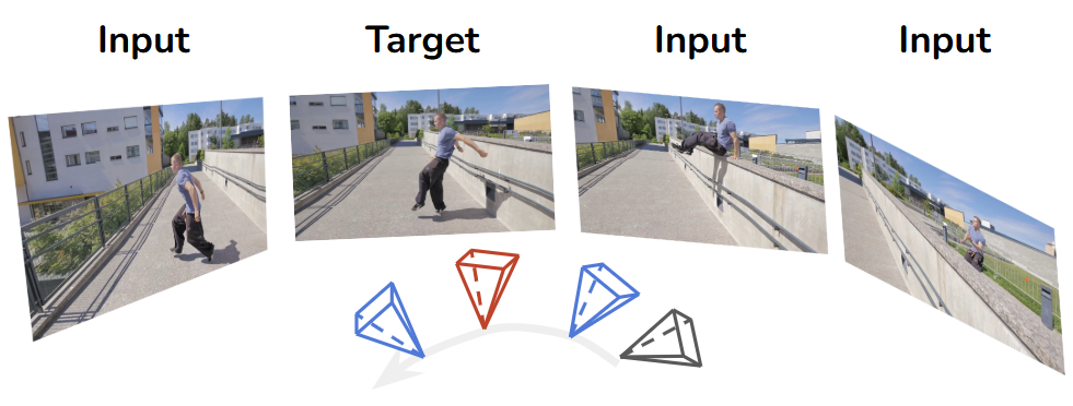
As a concrete testbed, I focus on spatial memory and 4D reconstruction (Believe it or not, this is more computationally doable and better defined than language modeling). I consider 4D novel view synthesis (NVS): given a long stream of posed views observed at different timestamps, the model is tasked with synthesizing novel views at new pose-time combinations. This plays a different role from text-only memory benchmarks like phonebook lookup or needle-in-a-haystack. Those tasks are, by design, almost pure match-and-retrieve: the model only needs to locate and replay a specific substring from a long context, which makes them excellent probes of pointer-like addressing capacity. In 4D reconstruction, by contrast, there is nothing to copy verbatim. The model has to fuse many observations into a consistent 4D scene representation and then render new views that were never seen before. Working memory is not just a pointer into the past context; it is a latent state that must be constructed, maintained, and queried.

Preliminaries

Fast Weights and Test-Time Training (TTT)

Test-Time Training (TTT)5 introduces a set of fast weights6 that are updated not only during offline training, but also online at inference time. 5 Learning to (Learn at Test Time): RNNs with Expressive Hidden States (Sun et al., 2024) 6 Linear Transformers Are Secretly Fast Weight Programmers (Schlag et al., 2021) This stands in contrast to conventional slow weights (the base model parameters), which remain fixed once training is finished. In the attention setting, we consider a sequence of tokens $$ \mathbf{x} = [x_1, x_2, \dots, x_N], $$ where each token is projected into key, query, and value vectors $$ x_i \mapsto (k_i, q_i, v_i). $$

TTT defines a small network or transformation $f_{\boldsymbol{\theta}}(\cdot)$ parameterized by fast weights $\boldsymbol{\theta}$. Each step consists of an update followed by an apply operation. Given a key-value pair \((k, v)\), the update rule takes a gradient step on a local loss: $$ \boldsymbol{\theta}' = \boldsymbol{\theta} - \eta \, \nabla_{\boldsymbol{\theta}} \mathcal{L}\big(f_{\boldsymbol{\theta}}(k), v\big), $$ where $\eta$ is a learning rate and $\mathcal{L}(\cdot,\cdot)$ encourages the transformed key $f_{\boldsymbol{\theta}}(k)$ to align with the value $v$. Intuitively, this trains the fast-weight module to compress the growing KV cache into a fixed-size neural memory, keeping important key-value associations while discarding the rest.

After the update, the apply step uses the updated fast weights $\boldsymbol{\theta}'$ to process a query $q$: $$ z = f_{\boldsymbol{\theta}'}(q), $$ yielding an output vector $z$ that depends on both the current query and the history encoded in the fast weights. A per-token TTT layer simply iterates these update/apply steps over the sequence.

Large-Chunk Test-Time Training (LaCT)

Naïve, per-token TTT is conceptually clean but hardware-inefficient: each update operates on an extremely small batch, which makes it hard to scale to long sequences or large models. Large-Chunk Test-Time Training (LaCT)7 addresses this by switching from token-wise to chunk-wise updates. 7 Test-Time Training Done Right (Zhang et al., 2025)

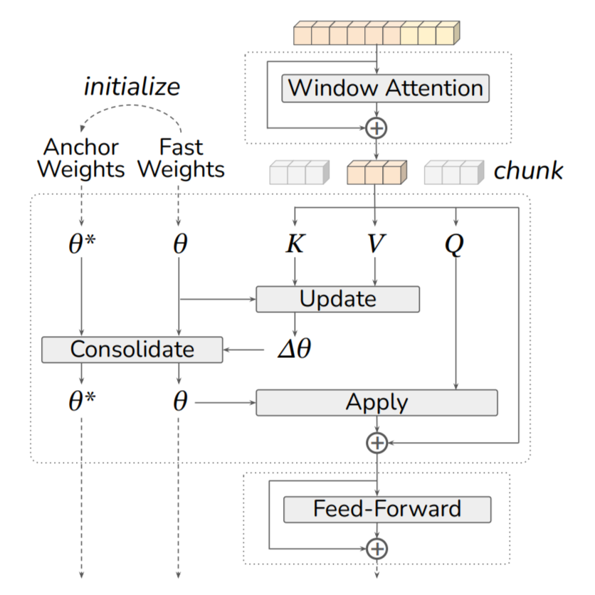
In LaCT, we group tokens into chunks of size $b$. All queries in a chunk share the same fast weights $\boldsymbol{\theta}$ for the apply step: $$ o_i = f_{\boldsymbol{\theta}}(q_i), \quad i = 1, \dots, b. $$ Instead of updating $\boldsymbol{\theta}$ after every token, LaCT aggregates a surrogate loss over the entire chunk and computes a single pseudo-gradient: $$ \boldsymbol{\theta} \leftarrow \boldsymbol{\theta} \; \underbrace{ - \; \nabla_{\boldsymbol{\theta}} \sum_{i=1}^{b} \eta_i(x_i)\, \mathcal{L}\big(f_{\boldsymbol{\theta}}(k_i), v_i\big) }_{\text{per-chunk surrogate pseudo-gradient}}, $$ where $\eta_i(x_i)$ are (optionally learned) per-token learning rates. Because each update now sees thousands of tokens at once, LaCT can amortize the cost of more expressive update rules (e.g., weight normalization, second-order preconditioning) and achieve much higher throughput than per-token TTT, while still behaving like a fast-weight learner over the sequence.

Large-Chunk Elastic Test-Time Training (LaCET)

In the original LaCT paper, authors observed that the model works best when we use a single large chunk per sequence. This can be interpreted as a form of inference-time bidirectional information sharing (credit to Haian Jin): the fast weights see all frames in the sequence at once, so updates can implicitly use information from both past and future views before producing the final predictions.

However, it misses the original ambition to handle arbitrarily long sequences in one streaming pass. With a single chunk, the effective context is still bounded by that chunk size. To truly move toward unbounded sequences, we have to allow the fast weights to be updated continuously across multiple chunks, not just once.

My hypothesis is that LaCT updates remain fully plastic, as the fast weights in each chunk drift freely in parameter space at inference time. To address this, we can draw on ideas from classic continual learning.

Elastic Weight Consolidation (EWC)

EWC8 introduces a quadratic penalty that discourages important parameters from drifting too far from a reference set of anchor weights, originally designed for a classic continual learning setting where a model learn a new task $\mathcal{T}_B$ without forgetting a previously learned task $\mathcal{T}_A$. 8 Overcoming Catastrophic Forgetting in Neural Networks (Kirkpatrick et al., 2016) All knowledge about $\mathcal{T}_A$ is captured in the posterior distribution $p(\boldsymbol{\theta}\,|\,\mathcal{D}_A)$. Since this posterior is intractable for large neural networks, EWC approximates it using a Gaussian centered at the previously optimized parameters $\boldsymbol{\theta}_A^{\star}$ with a diagonal precision given by the Fisher Information Matrix $F$, i.e., $p(\boldsymbol{\theta}\,|\,\mathcal{D}_A) \approx \mathcal{N}\!\big(\boldsymbol{\theta}_A^{\star}, F^{-1}\big).$ The Fisher Information has three desirable properties:

• It corresponds to the local curvature of the loss near $\boldsymbol{\theta}_A^{\star}$;
• It can be estimated from first-order gradients alone;
• It is guaranteed to be positive semi-definite.

Under this approximation, the total objective when learning $\mathcal{T}_B$ becomes a combination of the new-task loss and a quadratic penalty centered at $\boldsymbol{\theta}_A^{\star}$: $$ \mathcal{L}(\boldsymbol{\theta}) = \mathcal{L}_B(\boldsymbol{\theta}) + \sum_i \frac{\lambda}{2}\, F_i\, \big(\theta_i - \theta_{A,i}^{\star}\big)^2, $$ where $\mathcal{L}_B(\boldsymbol{\theta})$ is the loss for the new task $\mathcal{T}_B$, $\lambda$ controls the relative importance of retaining old knowledge, and $i$ indexes each model parameter. Intuitively, parameters with high Fisher values $F_i$ are crucial for $\mathcal{T}_A$ and are therefore strongly constrained to remain near $\boldsymbol{\theta}_A^{\star}$, whereas parameters with small $F_i$ can adapt freely to $\mathcal{T}_B$.

Elastic Test-Time Training (ETTT)

In our ETTT formulation, we reinterpret this idea at test time: each incoming chunk of data acts as a new task $\mathcal{T}_B$, and the fast-weight state from the previous chunk plays the role of $\boldsymbol{\theta}_A^{\star}$. The Fisher-weighted penalty thus serves as a continuously updated elastic prior, stabilizing the model's adaptation over time (e.g., foreground dynamics) while preserving useful past information (e.g., static background).

Formally, let $\boldsymbol{\theta}$ denote the LaCT fast weights within a given chunk, and $\boldsymbol{\theta}^\star$ their corresponding anchor parameters (the reference state before adaptation or at the last re-anchor). The EWC penalty defines an elastic prior after the LaCT update, which we refer to as the consolidate operator: $$ \boldsymbol{\theta} \;\leftarrow\; \boldsymbol{\theta} \; \underbrace{ -\; \lambda\, F \odot (\boldsymbol{\theta} - \boldsymbol{\theta}^{\star}) }_{\text{elastic consolidation}}, $$ where $\boldsymbol{\theta}^{\star}$ denotes the anchor (reference) weights, $F$ is a diagonal Fisher-style importance estimate, $\odot$ denotes the Hadamard (elementwise) product, and $\lambda$ is a constant controlling the strength of the elastic prior (step size absorbed).

Fisher Estimates

We maintain a per-parameter importance matrix $F_c$ as an EMA with decay $\alpha \in [0,1)$ over chunk index $c$: $$ F_{c+1} \;=\; \alpha\, F_c \;+\; (1-\alpha)\, \varphi\!\big(\mathbf{S}_c\big), $$ where the choice of statistic $\mathbf{S}_c$ and reduction $\varphi(\cdot)$ depends on the desired estimate. Let $\tilde{\mathbf{g}}_c$ denote the (pseudo-)gradient used by LaCT in chunk $c$, and let $\Delta\boldsymbol{\theta}_c = \boldsymbol{\theta}_c - \boldsymbol{\theta}_c^\star$ be the displacement from the current anchor parameters. Besides EWC, we also consider 2 alternative estimates, motivated by memory-aware synapses (MAS9) and synaptic intelligence (SI10). 9 Memory Aware Synapses: Learning What (Not) to Forget (Aljundi et al., 2017) 10 Continual Learning Through Synaptic Intelligence (Zenke et al., 2017) $$ \mathbf{S}_c = \begin{cases} \tilde{\mathbf{g}}_c, & (\textrm{MAS / EWC}) \\ \tilde{\mathbf{g}}_c \odot \Delta\boldsymbol{\theta}_c, & (\textrm{SI}) \end{cases} $$ $$ \varphi(\mathbf{S}_c) = \begin{cases} \lvert \mathbf{S}_c \rvert, & (\textrm{MAS / SI}) \\ \mathbf{S}_c^{\;2}, & (\textrm{EWC}) \end{cases} $$

Note that in the original SI formulation, $\Delta\boldsymbol{\theta}_c = \boldsymbol{\theta}_c - \boldsymbol{\theta}_{c-1}$. Under the LaCT update rule, this displacement is approximately proportional to the (pseudo-)gradient in each chunk, so the SI importance $\lvert \tilde{\mathbf{g}}_c \odot \Delta\boldsymbol{\theta}_c \rvert$ degenerates to a rescaled squared-gradient statistic, making it effectively equivalent to our EWC-style estimator in this setting.

Anchor Update Policies

ETTT allows different anchoring policies that control how $\boldsymbol{\theta}^\star$ is maintained:

• Global: anchors remain fixed to initialization, enforcing absolute stability;
• Streaming: anchors update at each chunk boundary, ensuring local temporal continuity;
• Streaming-EMA: anchors are updated via an exponential moving average (EMA11), $\boldsymbol{\theta}^\star \leftarrow \beta \boldsymbol{\theta}^\star + (1-\beta)\boldsymbol{\theta}$, forming a low-pass filter over the fast-weight trajectory. 11 Mean teachers are better role models: Weight-averaged consistency targets improve semi-supervised deep learning results (Tarvainen and alpola, 2017)

We will show later that Streaming-EMA is the best practice to ensure genuinely elastic memory behaviors.

Ablation Studies

Experiment Setups

We train a pose-conditioned 4D-LVSM (same encoder as 4D-LRM12 and same decoder as LVSM13) exclusively on internet stereo videos from Stereo4D14 dataset, trimmed to a maximum temporal window of 136 frames. 12 4D-LRM: Large Space-Time Reconstruction Model From and To Any View at Any Time (Ma et al., 2025) 13 LVSM: A Large View Synthesis Model with Minimal 3D Inductive Bias (Jin et al., 2025) 14 Stereo4D: Learning How Things Move in 3D from Internet Stereo Videos (Jin et al., 2024) The photometric training loss combines $\ell_2$ (MSE) loss and LPIPS loss. All ablation models use a 12-layer LaCET backbone with SwiGLU-MLP (w/o bias terms) as the fast weight network, trained with a per-GPU batch size of 16 on 8 H100 GPUs, using 32 input and 32 target views, a maximum temporal span of 128 frames, and an image resolution of $128 \times 128$ for 32K steps ($\approx$50B tokens). We deliberately use a small network so that its long-context performance saturates with a reasonably small number of tokens.

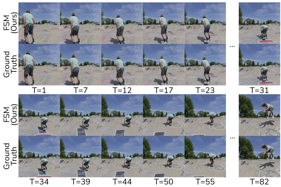
We evaluate on the Stereo4D test set using 136-frame clips, measuring PSNR/SSIM/LPIPS, using 32 randomly sampled views along the trajectory as inputs and averaged over 8 randomly sampled target views per scene.

Anchor Update Policies

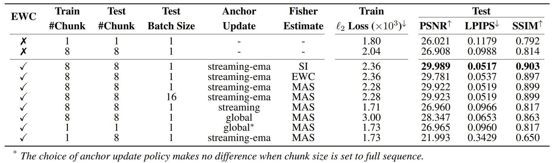
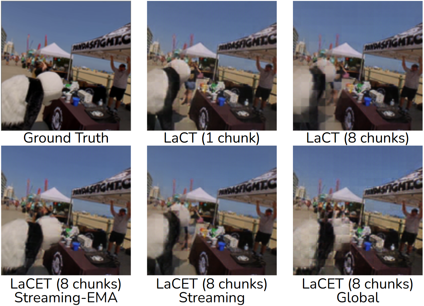
We first look at how the anchor weights are updated. Intuitively, the anchor is our reference fast-weight state, and EWC pulls the current fast weights back toward this anchor with a strength proportional to their estimated importance (the Fisher term). Different anchoring policies lead to very different behaviors.

Full-sequence setup (single chunk).
First, consider the simplest case: we treat the entire sequence as a single chunk. The model runs exactly one forward pass and one fast-weight update per scene. In this regime, all anchoring choices collapse to essentially the same behavior, because there is only one update step. Mathematically, the EWC term just adds a small higher-order correction on top of the LaCT update when the regularization strength $\lambda$ is small, so its effect is negligible. When $\lambda$ is large, EWC mostly behaves like a temporal low-pass filter or a form of weight decay applied to the inference-time learning: it damps very aggressive fast-weight changes, but there is no real notion of elastic memory over time, because the model only updates once.

Global anchoring.
In global anchoring, we fix the anchor weights once and never move them. EWC then degenerates into a static $\ell_2$ penalty that always pulls the fast weights back toward this global reference. In other words, EWC acts like a prior-stabilization term or classical weight decay on the fast weights, independent of any temporal structure in the sequence. This can prevent the fast weights from drifting too far, but it does not really implement a rich notion of elastic memory; it just says "don't move too far from the initial state."

Streaming anchoring.
In streaming anchoring (without EMA), we reset the anchor to the current fast weights at the start of each chunk. Within that chunk, EWC penalizes how far the fast weights move away from this freshly set anchor, effectively shrinking the within-chunk drift. However, once we move to the next chunk, the anchor is reset again, and there is no mechanism to consolidate what was learned in the previous chunk into a longer-term memory. As a result, this policy regularizes each chunk in isolation but does not accumulate knowledge across chunks. It behaves like a dynamically memoryless system: the model adapts and shrinks back inside each chunk, but there is little sense of slow, cross-chunk memory formation, and the risk of overfitting to local chunk statistics remains high.

Streaming-EMA anchoring.
The most interesting behavior emerges when we combine streaming anchors with an EMA update and squared Fisher estimates. Here, the anchor is no longer fixed or reset hard; instead, it evolves smoothly over time as a low-pass filtered version of the fast-weight trajectory. The EWC term then acts as an importance-weighted constraint on cumulative drift relative to this slowly changing anchor. Conceptually, this gives us genuinely elastic memory: the fast weights are free to adapt to new chunks, but important directions (as measured by the Fisher statistic) are softly tied to a consolidated anchor that carries forward past structure. The anchor moves, but it moves slowly; the fast weights can stretch away from it, but the elastic pull strengthens where the model has previously decided "this direction really matters."

Elasticity Improves Generalization

We observe a clear gap between training and test PSNR values of LaCT (i.e., training vs. validation $\ell_2$), indicating overfitting. Intuitively, plain LaCT seems to latch onto local shortcuts: it uses its limited fast-weight memory to memorize highly specific patterns, rather than maintaining a robust, distributed spatiotemporal representation of the scene. Our ablations show that this generalization gap can be mitigated by properly configured ETTT, but this also motivates us to ask...what does LaCT overfit to in the 4D NVS task?

Memory vs Interpolation

We compare how LaCT and LaCET behave under different test-time input densities. Both models are trained with 32 input images, and we vary the number of input frames at inference on 136-frame Stereo4D clips.

• Discrete-view setting: input and target frames are uniformly sampled across the full span;
• Continuous-view setting: we crop a contiguous sub-sequence (e.g., 40 frames for the 32-in/8-out case) and mask the target frames within that window, reducing the problem to frame interpolation.

Two settings converge when the full 136-frame span is used.

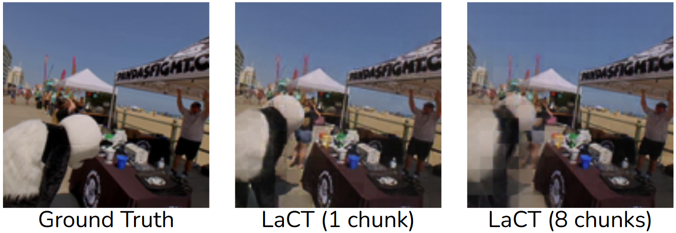
When input views are sparse in time and space, LaCET has a clear and systematic advantage over LaCT across PSNR/SSIM/LPIPS. With 8 chunks, both LaCET and LaCT degrade as we make views sparser, but LaCET stays noticeably stronger. LaCT with a single chunk degrades more gracefully because it spends far more activation memory to process the full sequence at once, which is not sustainable for truly long streams. Smaller chunks remain attractive because they reduce activation memory (backprop spans fewer samples) and are therefore much closer to a realistic streaming setup.

LaCT only catches up in the continuous-view regime with large chunks. When inputs become dense and continuous in time, LaCT with larger chunks starts to regain performance and can even approach LaCET, while LaCT with 8 small chunks still lags behind. Our interpretation is that LaCT is mainly exploiting short-range temporal redundancy: when frames are continuous, the task effectively collapses to frame interpolation. Mitchel et al.15 made similar observations. The model can lean on neighboring frames inside the context window and no longer needs to perform genuine 4D novel view synthesis, such as extrapolating to unseen camera poses or maintaining long-range temporal structure. 15 True Self-Supervised Novel View Synthesis is Transferable (Mitchel et al., 2025)

Final Remarks

A key simplifying assumption behind a lot of discussion in this space is the idea that "parameter count = memory capacity." However, equating parameters with memory capacity blurs an important distinction between storing information and using it. A model can, in principle, memorize a huge corpus in its weights and still fail at tasks that require composing knowledge, abstracting patterns, or performing multi-step reasoning. Those abilities live in the circuitry implemented by the parameters, i.e., the algorithms the network has learned to run, not just in how many bits of past data it can implicitly cache.

LaCET is my attempt to make the inference-time part of the picture more explicit. At the end of the day, it can still be viewed as a kind of linear attention model: it compresses long histories into a fixed-size state that can be updated and queried in a streaming fashion. Like other linear or kernelized attention mechanisms, my working hypothesis is that LaCET will shine on memory-intensive tasks that demand stable access to a large amount of information over long sequences, especially in settings like 4D reconstruction where the target signal is geometrically well-defined. I do not expect this architecture alone to suddenly solve tasks that require deep multi-step reasoning, counterfactuals, or subtle abstraction. Long working memory is necessary for those behaviors, but it is almost certainly not sufficient.

More broadly, this line of work is less about claiming a final solution and more about carving out a cleaner factorization: separate the question of how much information a model can reliably carry forward in one pass from the question of what computations it chooses to perform over that information. If we can design architectures where activation memory no longer scales with sequence length, we can probe working memory limits without immediately hitting hardware limits. Once that bottleneck is relaxed, we can start asking sharper questions about controllers, reasoning procedures, and how to couple these memory systems to agents that act in the world.

The full model and code will be released once the paper review process is complete. Stay tuned.

Citation

To give credit if you find this work useful, please cite:

@article{ma2025fast,
  title={Fast Spatial Memory with Scalable Elastic Test-Time Training},
  author={Ma, Ziqiao and Yu, Xueyang and Zhen, Haoyu and Yang, Yuncong and Chai, Joyce and Gan, Chuang},
  journal={https://mars-tin.github.io/},
  url={https://mars-tin.github.io/blogs/posts/elastic_ttt.html},
  year={2025}
}